Ch. 1
Ch. 2
Ch. 3
Ch. 4
Ch. 5
Ch. 6
Ch. 7
Ch. 8
Ch. 9
Ch.10
Ch.11
Ch.12
App.1
App.2
App.3
Biblio.
Index
Hector Parr's Home Page
Quantum Physics: The Nodal Theory
Hector C. Parr
Chapter 3: Probability and Quantum Amplitudes
3.02 Probability plays an even bigger part in Quantum Mechanics, for almost all events and processes seem to involve an element of randomness. When conducting an interference experiment we can have no idea where a particular particle will strike the screen, but can often specify accurately the probabilities of its arriving within different specified areas. When a photon approaches a pair of polarising filters we cannot know in advance whether it will be transmitted or absorbed, but when a large number of photons are involved we can calculate with precision the proportion which will be transmitted, and hence the probability that an individual photon will be. We have no idea when a radio-active nucleus will disintegrate, but we know accurately the probability that such a nucleus will do so in any given time interval, from which we can calculate the half-life of a sample containing a large number of atoms, and the proportion remaining after any required time.
3.03 The question of whether quantum phenomena also exhibit apparent randomness only because they are determined by hidden variables of which at present we have no understanding, or whether they are truly random in a way that macroscopic systems never are, was vigorously debated during the second quarter of the twentieth century. In particular the famous discussion between Niels Bohr, who was the chief spokesman for the most widely held views on the interpretation of quantum phenomena, and Albert Einstein, who was convinced that quantum behaviour would indeed prove to be deterministic when we discovered the hidden variables which dictated its apparent randomness, provided a fascinating example of great brains wrestling with a difficult problem. Although the argument was not resolved during the lifetime of either man, the depth of thinking which it evoked on both sides did much to clarify our ideas. Today, in the light of experimental developments which have occurred since Einstein’s death in 1955, it seems likely that he was on the losing side. Einstein refused to accept two of the most strange aspects of Bohr’s viewpoint, the indeterminacy of quantum behaviour, and the apparent transmission of influences at speeds greater than that of light. This latter principle, which has come to be known as “non-locality”, seemed at the time to violate the dictates of Special Relativity. But during the last quarter of the twentieth century many experiments appear to have shown that we cannot escape from non-local influences even if we accept that their randomness is a result of hidden variables. It is likely that Einstein would have admitted defeat in view of this more recent evidence, for it seems impossible to describe the quantum world wholly in terms of classical principles, as he had hoped. But whether or not quantum phenomena are really random, we must still use the methods of probability theory to describe them, just as we do for macroscopic behaviour which is not truly random, such as that of coins and dice.
3.04 The concept of probability is much more difficult to define than most people imagine, and no branch of mathematics provides more fertile ground for misunderstanding and paradox. Sometimes the results are amusing, as when we seem to find several different answers, all plausible, to the same problem. Sometimes they are frustrating, and throughout the twentieth century the interpretation of Quantum Physics has been hampered by misunderstandings and lack of clarity in the application of probability theory. But sometimes they can be disastrous, as when they give rise to miscarriages of justice which commit innocent people to long prison sentences. We shall illustrate all these types of mistake in a later section of this chapter. In order to prevent ourselves making similar mistakes it is necessary to study the concept of probability in some detail.
3.05 We use the techniques of probability theory only in relation to propositions or events about which we have incomplete knowledge, usually because they lie in the future. If we knew exact details of everything that has ever happened or ever will happen, probability would no longer be necessary or meaningful. It follows that any value we quote for the probability of an event is relative to some corpus of knowledge that we have about that event, or that we choose to hypothesise about it, and will change if that knowledge changes. It is often supposed that an event can have an intrinsic probability, a property possesed by that event, just like the time or place of its occurrence, but this belief shows a fundamental misunderstanding. Probability is merely a relationship between an event and one person's knowledge of that event. The value of a probability may well differ for different people, and may differ for one person at different times, as that person gains additional knowledge of the event. This answers the rather silly question of whether the odds of a coin landing “heads” remains 1:1 after we have actually seen how it landed. If we choose to use the additional knowledge we have after looking at it, then the probability of a head becomes 0 or 1, as the case may be. If we do not, then it remains 1/2.
3.06 Attempted definitions of probability may be described either as “subjective”, if they refer only to a particular person's beliefs regarding unkown or future events, or “objective”, if framed in terms of the actual occurrences of such events themselves. Mathematicians seem to prefer objective definitions, while philosophers are more likely to subscribe to the subjective. The philosopher often thinks of the probability of event A as his “degree of rational belief that A will occur”, an interpretation particularly associated with Maynard Keynes (1883-1946) and Rudolf Carnap (1891-1970). Thus he may claim to be “one half certain” that the coin will land heads, or 1/52 certain that he will draw the Queen of Hearts. The writer cannot accept this as a definition. Surely we cannot have “degrees of belief”. There are some propositions which I believe to be true, and some that I believe to be false, but if I am convinced neither one way nor the other about a proposition then I have no belief concerning it. I cannot be certain that the next throw of the coin will result in a head, and so I do not believe that it will, and nor do I believe that it will result in a tail; maintaining that one can have “half a belief” is an attempt to divide the indivisible. Those who claim to have “degrees of rational belief” are using the word “belief” in a sense that I do not understand. The phrase sounds plausible at first, but those who use it really mean something different, probably something nearer to the mathematical definition of probability, but which they cannot put into words because of unfamiliarity with mathematical notation and convention.
3.07 One attempt to overcome this kind of objection is provided by the "principle of indifference". This proposes that if we have no reason to believe one proposition rather than another, we should assign them equal probabilities. It is easily seen, however, that this is untenable because of the inconsistencies it entails. Suppose you pick three names at random from a telephone directory, Mr. A, Mr. B and Mr. C. You have no reason to know whether B is shorter or taller than A, so by the principle of indifference you assign equal probabilities to the two propositions. In other words, the probability that B is shorter than A is one half. By a similar argument, the probability that B is taller than C is also one half. It follows that the three persons, in order of increasing height, cannot be A, B, C, for B must either be shorter than A or taller than C. This is absurd, and shows that our original premise, the principle of indifference, is false.
3.08 Another approach is the “Personalism” of Bruno de Finetti (1906-1985) and Frank Ramsey (1903-1930), defining the probability a person attributes to a certain event in terms of the betting odds he would wager on it. Again this is too vague to furnish a reliable definition, for people differ widely in their readiness to take risks. Some young men will stake their lives on the belief that they can control their cars at speeds which are clearly too high, while some older people will not venture out of doors for fear of being attacked. This is no basis for assessing the probability of being involved in road accidents or becoming victims of crime.
3.09 In fact it seems that no truly subjective definition of probability is viable, for such a definition must be derived at some level from an objective one. It is mistaken to think we know a priori that a coin lands heads with probability 1/2. We have already had some experience, however remote, of probability defined mathematically, and hence objectively. We claim to be one-half certain the coin will land heads only because we can visualise it being tossed repeatedly, and know that the number of heads is likely to be about one half the number of throws, or alternatively because we understand that one half of the coin's possible starting conditions lead to a head.
3.10 If we are thus driven to define probability mathematically rather than subjectively, why should this prove difficult? There are many situations, in gambling and elsewhere, when the probability of some event is obvious, with no room for disagreement. As an example, suppose you are asked for the probability of throwing an even number when a dice is rolled. You know there are six possibilities, of which three are even, so the probability must be 3/6, or 1/2. So let us ask what are the distinguishing features of situations in which probabilities are fairly obvious. Firstly, they must be repeatable. We can roll a dice as often as we like, and this is what we would do if our assertion of the above probability were challenged. When a possible situation is totally unique, and cannot be repeated, it is meaningless to ascribe to it a probability, for how could we ever confirm that the value we give it is correct? Secondly, situations governed by probability always involve an event (in this case the throwing of an even number) which, in different trials, sometimes happens and sometimes does not. In many such situations, the proportion of trials in which the event happens, while it can take any value between 0 and 1, is found to concentrate around some particular value as the number of repetitions increases. This is the value we have in mind when the probability of an event seems obvious. Thirdly, while each trial may result in any one of a number of outcomes (in this case six), the event itself is related to a particular subset of these outcomes, in this case 2, 4 or 6.
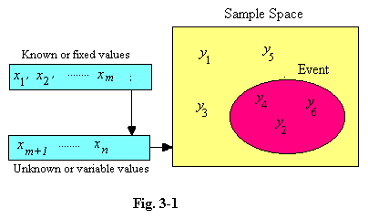
3.11 We can illustrate these facts on a diagram. The initial conditions, or the given situation, may be represented as the values of n variables, x1 to xn. We suppose that the first m
of these (e.g. the size and shape of the dice) are held constant during
all the trials, while the others (e.g. the position and speed of the
throw) are allowed to vary unpredictably. Thus xm+1 to xn
are the hidden variables, and if we deny the existence of these in
quantum situations, all the variables are fixed. We represent the
outcomes of the trials by y1, y2, ... , and the
set of all possible outcomes (in this case 1, 2, 3, 4, 5 or 6) we call
collectively the “sample space”. The event E (e.g. the throwing of an
even number) comprises a particular subset of the outcomes (2, 4 or 6).
Our first attempt at an objective definition relies on the fact that the possible outcomes of an experiment, which we have represented by y1, y2 ..., will often be equally likely. The six possible results when a dice is rolled satisfy this condition, provided the dice is not loaded. Then if there are s equally likely ways in which an event can occur, and r of these are “successful”, the probability of success is r/s. In such cases this would seem to provide an unambiguous meaning for “the probability of the event occurring”. The trouble is that the definition is useless because it is circular; “equally likely” is just another way of saying “equally probable”. Our definition of probability is meaningful only if we know already what probability means.
3.12 A
second approach to the problem is to use a method known as “range
theory”. The result of a trial is often uniquely determined by the
values of the variables m+1 to n in the diagram above,
and we suppose these to vary randomly. Can we not define the
probability of “success” by expressing the range of possibilities of
these n-m variables under which success is achieved as a
proportion of the total range of possibilities? In other words, can we
not take the average value, with success counting as 1 and failure as
0, averaged over these random variables? Unfortunately no; not with any
certainty that the method will yield a unique value. It has long been
known that this range method can lead to conflicting values for the
same probability, and a good example of this was described by J.
Bertrand (1822-1900) in 1889.
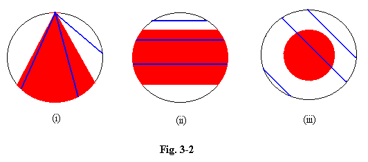
3.13 He asked what is the probability that a chord drawn at random in a circle is longer than the side of an equilateral triangle inscribed in the same circle. If we consider all chords drawn through a particular point on the circumference (see (i)), the condition is satisfied only by those chords which make an angle of less than 30 degrees with the radius through that point, out of a total possible range of 90 degrees, so the required probability must be 1/3. But if instead we consider all the chords drawn perpendicular to a given diameter (see (ii)), the condition is satisfied whenever the centre of a chord is less than half a radius from the centre, so the required probability must be 1/2. Or thirdly, we can see that the condition requires the centre of the chord to lie within a circle of radius one-half that of the given circle, i.e. within a circle of area one quarter of the given circle (see (iii)). So the probability must be 1/4. A definition which gives three different answers to the same question is clearly unacceptable. Despite the fact that many writers believe range theory to provide a sound definition, and a means of determinig probability values in practice, we must reject it for either purpose because of its unreliability.
3.14 Both of the above methods of assigning probabilities may be described as a priori, for they depend upon knowledge we have of a system before conducting any trials. A third method, the empirical method, defines probability in terms of the actual frequencies observed when a practical experiment is performed many times, rather than by consideration of causes. This approach is associated with John Venn (1834-1923), but this too is not without difficulties. Let s denote the number of trials, and r the number of “successes”, and define probability as the observed value of r/s. This is easily seen to be unsatisfactory, for it will give a different value each time the experiment is repeated, and will seldom give the value we know intuitively it should. If a coin is tossed 1000 times it is unlikely the number of heads will be exactly 500: it is almost equally likely to be 510 or 520, giving values of 0.51 or 0.52 for the probability which we know ought really to be 0.50. We might claim that we can always get as close as we wish to the correct value by repeating the experiment a sufficient number of times, but this also is false. If the coin is tossed a million times it is true that 510000 heads are unlikely, but they are not impossible. Indeed if the million tosses are themselves repeated a sufficient number of times, we can calculate when it will become more likely than not that at least one of the attempts will yield 510000 heads. We cannot be sure of getting as close as we wish to the correct answer by any pre-specified number of trials, however great.
3.15 We can attempt to put the above method on a firmer mathematical footing by defining the probability not as the value of r/s, but as the limit of r/s as s tends to infinity. But this fails equally, for it can be shown that if the sequence of successes and failures is truly random, then r/s does not, in fact, tend to a limit. The strict meaning of “r/s tends to the limit p as s tends to infinity” is that, given any small number q, a value so for s can be found such that r/s differs from p by less than q for all values of s > so. Clearly this will never be true; it is always possible for a run of successes to occur long enough to raise the value of r/s, or a run of failures to lower the value of r/s, so that it lies outside the limit prescribed. Nonetheless, if we ignore this difficulty, and try to assess a limiting value by observing a long series of trials, we shall usually obtain a result close to the correct one. The error could, in fact, be of any magnitude, but with a sufficiently long sequence, it will be substantial only very rarely.
3.16 The previous section has provided three possible definitions of probability. Each is imperfect in some respect, as we have shown, but each does sometimes give a useful method of finding probability values in practical investigations, with little risk of error.
3.17 The occurrence or non-occurrence of an event E depends upon which of the y alternatives occurs, as our diagram shows. Often we have good reason to believe that these alternatives are all equally likely (while realising we cannot put this belief on a firm logical footing), and then we know the probability of E will be the proportion of these alternatives which entail E. The symmetry of a dice or a coin is sufficient reason to allow us to believe the outcomes to be equally likely when we roll a dice or toss a coin. The probabilities of various combinations of result are then easy to calculate.
3.18 In reaching this conclusion we are unthinkingly making use of range theory. The result of spinning a coin obviously depends upon the speed with which it is spun, and because we cannot accurately control this speed we assume an equal likelihood for heads and tails. This is reasonable because we know a small difference of speed can cause a large difference in the number of times the coin turns over while in flight.
3.19 But there are often cases in which an analysis of causes gives little guide to the probabilities we are attempting to find, and in such cases we must rely on the empirical method. We conduct a large number of trials, and assume the probability to equal the proportion of outcomes which are “successful”. Thus, to find the probability that a single photon arrives within a particular region of the screen in an interference experiment, we observe a large number of photons, all prepared in the same way, and we note the proportion which arrive in this region. Notice that, if we reject the “hidden variable” theory, we can indeed prepare our photons all in the same state, in contrast with what happens in corresponding macroscopic experiments. When tossing a large number of coins we cannot ensure that they all have the same starting conditions; the variables xm+1 to xn are outside our control. But in the quantum case these values do not exist; if we reject hidden variables, then m = n, and all the initial conditions can be determined by the experimenter.
3.20 It is necessary to emphasise again that the value of a probability assigned by a person to a particular event depends on that person's imperfect knowledge of the event. If you know that the four Aces have been removed from a pack of cards, for you the probability of drawing a Queen is 4/48, or 1/12, while for me it will remain 1/13. Neither of these values should be regarded as wrong; each is a correct evaluation based upon one person's knowledge of the situation. A simple error known as the “gambler's fallacy” illustrates the importance of specifying carefully what knowledge we are taking into account. If a coin has been observed to fall heads on ten successive occasions, many people believe wrongly that the likelihood of a head on the eleventh throw is then less than 1/2, because of what they call the “law of averages”. Such people are confusing two questions. If a coin is tossed eleven times and we know none of the results, the probability of all eleven being heads is less than 1 in 2000. But if we know that the first ten results are indeed heads, then the probability of the eleventh also being a head is just 1/2 as always.
3.21 Not
only the ignorant can make such errors. The renowned physicist Paul
Davies describes a simple experiment in which a stream of electrons
builds up an interference pattern on a screen, and writes,
These results are so astonishing that it is hard to digest their significance. ... How does any individual electron know what the other electrons ... are going to do? (Other Worlds, Penguin, 1980)The results are indeed surprising, but not for this reason. Does Davies ask how a coin knows which way it will fall on subsequent occasions? It is because the coin does not know, because its results are independent of each other, that the characteristic distribution of results is built up.
3.22 The knowledge we take into account may be just hypothetical; even if I know the pack to be complete I can still ask the question, “If the four Aces were missing what would be the probability?” In this type of question we are making an adjustment to the first set of x values in the diagram above, the “known or fixed” values. But it is important not to allow this to happen inadvertently; such errors account for many of the well-known paradoxes associated with probability theory.
3.23 A dangerous error arises when we fail to specify sufficiently clearly the event E whose probability we want. A good illustration is provided if we toss three coins, and ask what is the probability that they all fall showing the same face, i.e. all heads or all tails. There are clearly eight equally likely results, HHH, HHT, HTH, etc., and two of these satisfy our condition, namely HHH and TTT. The required probability is therefore 2/8 or 1/4. But what is wrong with the following argument? When we look at three coins, there must be two showing the same face. The probability that the third coin agrees with them is then 1/2, not 1/4 as we obtained previously. The trouble here is that we are not specifying E clearly; we do not know which two coins will be the same, nor whether they will be HH or TT, and so the requirement we are imposing on the third coin is not fixed either. While enquiring whether the third coin's y value lies within the event E we are shifting the goalposts through which we require it to pass.
3.24 Many paradoxes arise from carelessness in specifying the sample space within which a probability is to be determined. If Mr. Smith tells us he has two children, of whom the elder is a boy, we would rightly suppose the probability of the younger also being a boy to be 1/2. But if he tells us he has two children, one of whom is a boy (without saying which), the probability of the other being a boy is now 1/3, for our knowledge is different. The new sample space contains three equally likely possibilities, namely BB, BG and GB (in each case specifying the elder child first), only one of which meets the required criterion.
3.25 A serious mistake sometimes occurs in a court of law. Let us suppose a man living in England is accused of a murder or a rape. The only evidence against him is a sample of bodily material left at the scene of the crime. If the forensic scientist tells the jury that this sample could have been left by only one person in a million, it is quite possible the defendent will be convicted on this evidence, for the jury are likely to conclude that the probability of him being innocent is only one in a million. In fact it is nothing of the sort. If we suppose a total adult male population of twenty million, then we can expect about twenty men to match the forensic sample. Only one of these men is guilty and the other nineteen are innocent, so the probability of the suspect being innocent, if no other evidence is available, is 19/20. The jury are not being asked to decide whether the suspect matches the sample; this piece of information is given. They are required to decide if he, among those who do match, is the one responsible for the crime. They mistook both the sample space and the subset of outcomes required.
3.26 The New Scientist journal (13 December 1997) quotes several cases in which a suspect has been found guilty on this sort of evidence, with neither the prosecution nor the defence noticing the fallacy. In one of these cases the accused had to serve a seven year jail sentence after the failure of two appeals.
3.27 Many people try to discuss the probability of hypothetical events which by their nature are unique, despite the fact that such a probability is meaningless. The actuaries employed by insurance companies work constantly with probabilities in assessing premiums. In most cases these probabilities will be determined by empirical methods; life insurance premiums are based on past statistics of life expectancy, and insurance against motor accidents or wet days will depend on past accident rates and weather records. But occasionally clients may seek cover for events which are essentially singular, in that no sequence of previous trials can exist. In these cases insurers must rely upon intuition. What would you expect to pay to cover the cost of rebuilding your London home if it is struck by a meteorite during the next fifty years, or replacing your workforce if it is captured by aliens from another planet? We never ought to talk about the probability of such events.
3.28 Our final example of a paradox is taken from Quantum Mechanics, and has engendered more than sixty years of argument. It concerns the “EPR” experiment devised by Einstein and two colleagues 1935, which seems to lead to impossible results whenever it is performed. While we admit that the results are unexpected, we maintain that the apparent contradiction arises from applying probability methods without defining properly the sample space involved. A full treatment will be found in a later chapter.
3.29 We have to use the methods of probability theory when solving problems at the atomic level because quantum systems are not deterministic. By this we mean that the present state of a system does not contain sufficient information to enable its future state to be calculated unambiguously. Experiments in particle physics are often conducted by preparing large numbers of identical particles in identical states. All the variables of which we are aware, such as position, momentum and spin, are set to identical values, so far as possible, and yet the particles do not all behave in the same manner, and the only way of relating their future performance to their present state is by means of probabilities.
3.30 The same applies to macroscopic systems, such as coins, dice or roulette wheels, which do behave deterministically, but whose behaviour is so complex that we cannot possibly know the values of all the relevant variables. The behaviour of elementary particles, however, displays an additional complication for which there is no parallel in the world of familiar experience. Ordinary probabilities are expressed as single numbers lying between 0 and 1, with 0 representing impossibility and 1 certainty. But many examples of quantum probabilities can be described only by using two numbers, or alternatively a two-dimensional vector. The best way to visualise such a vector is as a small arrow, such as one would use to represent a velocity or a force. The two numbers would then stand for the length of the arrow, taken to represent its strength or magnitude, and the angle it makes with some fixed direction such as the x-axis. The reason for this complication, and that an ordinary probability value will not suffice, lies in the fact that a quantum probability possesses, in a way which we cannot understand, a phase angle as well as a magnitude, and consideration of these phase angles plays an important part in the calculation of quantum effects, particularly in phenomena involving interference. So in describing a quantum probability we must quote both the magnitude and phase of such a vector. However, mathematicians often use an alternative description, and give us instead the x and y co-ordinates of the tip of the arrow, assumed to be drawn from (0,0) to (x,y), and they then go a step further and use just a single complex number, of the form z = x + iy, where i is the square root of -1. Non-mathematicians must believe us when we tell them that such a procedure does considerably simplify calculations involving these quantum amplitudes, or probability amplitudes, as they are called. (It is unfortunate that the y component of such quantities has come to be called the "imaginary" part. In fact it is just as real as the x component, and the vector represented by such a complex number can be just as real as the force you exert when dragging a piece of furniture across the floor. The only strange fact in the application of complex numbers to quantum mechanics is the need for two numbers rather than one.) When it is required to convert a quantum amplitude to an ordinary probability, we find that it can be done by squaring the length of our arrow, or the magnitude of the complex number. We write this as |z|2, and the value is given by the formula x2 + y2.
3.31 We often need to multiply probabilities together. If A and B are independent events, then the probability of the combined event “A and B” is found by multiplying together the probability of A and the probability of B. The probability of drawing a red card from a pack is 1/2, and the probability of drawing an ace is 1/13, and so the probability of a red ace is 1/2 multiplied by 1/13, which comes to 1/26. It can easily be seen that the same rule applies to quantum amplitudes. We can find the amplitude for a compound event, when we know that for each separate event, by multiplying together the two amplitudes, and then if we want the probability of the compound event, we just square its magnitude in the usual way. In fact it does not matter whether we multiply the magnitudes and then square the amplitude, or square the two separate amplitudes and then multiply, for it can be shown that |z1 X z2|2 = |z1|2 X |z2|2.
3.32 And we sometimes must add probabilities. If A and B are mutually exclusive events, then the probability of the event “A or B” is found by adding the probabilities of A and of B. The probability of drawing a spade is 1/4; so the probability of drawing a red card or a spade is 1/2 + 1/4, or 3/4. But we must be careful when dealing with the quantum amplitudes of two such events, for it is not true that |z1 + z2|2 = |z1|2 + |z2|2. In fact the corresponding rule for quantum amplitudes is much stranger. If we have set up an experiment in which we can determine not only that “A or B” occurs, but which of the two alternatives, then the same rule applies as with normal probabilities; we must find the separate probabilities by squaring magnitudes, and the final composite probability by adding these in the usual way. But if we know only that “A or B” occurs, and it is inherently impossible to know which alternative, we must add the complex amplitudes first, and then square the magnitude, or we get the wrong answer. This situation occurs, of course, in interference experiments, where particles have two or more possible routes to their destination, and where we cannot find out which route has been followed without destroying the interference effect, and to calculate probabilities we must add together the relevant probability amplitudes first and then find the squared magnitude. If instead we square the magnitudes separately and then add them together, we shall thereby lose track of the phase angles which determine the interference effects. This strange fact lies at the heart of the most perplexing quantum paradoxes, and the reader is urged to be certain it is fully understood before reading the remainder of the book.
(c) Hector C. Parr (2002)
Previous Next Home Hector Parr's Home Page